How to use nachos

Concepts

The numerical differentiation is used to obtain (static) derivatives to different quantities. It exploits the following identity, given \(f(x)\) a given function expanded in Taylor series,

\[\left.\frac{\partial f(x)}{\partial x}\right|_{x=0} = \lim_{h_0\rightarrow 0} \underbrace{\frac{f(h_0)-f(0)}{h_0}}_{\text{forward derivative}} = \lim_{h_0\rightarrow 0} \underbrace{\frac{f(h_0)-f(-h_0)}{2\,h_0}}_{\text{centered derivative}},\]

where \(h_0\) is the minimal field (min_field parameter).
The code use the Romberg procedure to remove contamination from higher orders (see this publication for more details). The derivative is computed for different values of \(h=a^k\,h_0\), with \(k<k_{max}\) the field amplitude (which lead to the k_max parameter), and \(a\) is the common ratio (ratio parameter). The procedure goes as follow:

\[\begin{split}\begin{align} &H_{k,0} = \frac{f(a^kh_0)-f(-a^kh_0)}{2\,a^kh_0},\\ &H_{k,m} = \frac{a^{2m}\,H_{k,m-1}-H_{k+1,m-1}}{a^{2m}-1}, \end{align}\end{split}\]

where \(m\) is the number of iterations (or refinement steps). This leads to a so-called Romberg triangle, from which the value of the derivative is extracted. The algorithm to select the best value is described in qcip_tools numerical differentiation page.
The different quantities are written as derivatives with respect to the energy. For example, the geometric Hessian, second order of the energy with respect to geometrical derivatives, is written GG, G meaning geometrical derivative with respect to cartesian coordinates. Accordingly,
- F means derivatives with respect to static electric field ;
- D means derivatives with respect to dynamic electric field (with a given frequency), d means the same, but with inverse frequency (\(-\omega\)) and X means any multiple (\(\pm i\omega\)) ;
- N means derivatives with respect to normal coordinates.
Therefore, the static hyperpolarizability, \(\beta(0;0,0)\), is written FFF, while the dynamic hyperpolarizability depends on the process involved: dDF for EOP [\(\beta(-\omega;\omega,0)\)] and XDD for SHG [\(\beta(-2\omega;\omega,\omega)\)]. See the list below.

Geometrical derivatives of an electrical derivative are written with the geometrical derivatives first. For example, the first order geometrical derivative (with respect to normal mode) of the static polarizability, \(\frac{\partial \alpha}{\partial Q}\), is written NFF, the second order one NNFF.

Note that the number of G and N thus correspond to the level of geometric differentiation and the number of F, D and d to the level of electrical differentiation.
Nachos is abble to perform differentiation with respect to static electric field (F) and cartesian coordinate (G). Given the cartesian hessian, nachos_bake (see below) perform a vibrational analysis and is able to project G derivatives over normal mode, giving the corresponding N ones.
Nachos (because of the underlying library, qcip_tools) takes advantage of permutation symmetry and Shwarz’s theorem (referred as “Kleinman symmetry” in the field of nonlinear optics).

General workflow

Here is the schematic of the workflow with the nachos package:

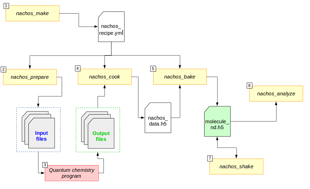
_images/workflow.png — Flowchart for the different parts of the nachos package. Arrows indicate whether a part is an input (arrows going in) of a program (rectangle) or an output (arrow going out).

In short,

nachos_make creates a recipe (nachos_recipe.yml, but you can change that), which is the file that explains what to do and how to do it ;
nachos_prepare uses the recipe to generate the different input files for the quantum chemistry program of your choice (currently Gaussian, Dalton and Q-Chem) ;
The quantum chemistry program process the different input files and generate output files ;
nachos_cook carry out all the information that it can get from output files (FCHK files for gaussian, TAR archives and OUT files for Dalton) and store them in a data file (nachos_data.h5, but you can change that) ;
nachos_bake perform the requested numerical differentiation(s) out of the data from the data file, and store them in a final file (molecule_nd.h5, but you can change that) ;
(optional) nachos_analyze allow to quickly get a given property for each quantity stored in the final file (e.g. a tensor component, an average, …). nachos_peek also allow you to do that, but it dumps everything ;
(optional) if possible, nachos_shake will add the different vibrational contribution to the electrical derivatives of the energy.

Therefore, it should looks like:

# create subdirectory:
mkdir new_directory
cd new_directory

# create recipe and inputs:
nachos_make && nachos_prepare

# ... run all the inputs ...

# carry out and perform numerical differentiation:
nachos_cook && nachos_bake # or nachos_bake -P

# ... eventually, add vibrational contributions:
nachos_shake

# ... eventually, post-analyze:
nachos_analyze -p "xxxx" > nachos.log
# ... and/or ...
nachos_peek molecule_nd.h5

See below for more details on every command.

nachos_make

Make a recipe

usage: nachos_make [-h] [-v] [-N] [-S] [--flavor FLAVOR] [--type TYPE]
                   [--method METHOD] [--basis-set BASIS_SET]
                   [--geometry GEOMETRY] [--differentiation DIFFERENTIATION]
                   [--frequencies FREQUENCIES] [--name NAME]
                   [--min-field MIN_FIELD] [--ratio RATIO] [--k-max K_MAX]
                   [--flavor-extra FLAVOR_EXTRA] [--XC XC] [--CC CC]
                   [--gen-basis GEN_BASIS] [-o OUTPUT]

-h, --help: show this help message and exit

-v, --version: show program’s version number and exit

-N, --fallback-prompt: do not use prompt_toolkit

-S, --stop-when-fail: fail when argument input is wrong

--flavor <flavor>: flavor for the recipe

--type <type>: type of differentiation

--method <method>: computational method

--basis-set <basis_set>: basis set

--geometry <geometry>: geometry of the molecule

--differentiation <differentiation>: quantities to differentiate

--frequencies <frequencies>: frequencies (if dynamic quantities)

--name <name>: Name of the files

--min-field <min_field>: Minimum field (F_0)

--ratio <ratio>: ratio (a)

--k-max <k_max>: Maximum k (k_max)

--flavor-extra <flavor_extra>: Update the values of flavor extra

--XC <xc>: XC functional (if DFT)

--CC <cc>: CC level (if CC)

--gen-basis <gen_basis>: gaussian basis function file (if gen)

-o <output>, --output <output>: Output recipe file

Note

It is easier to place the geometry file (and eventual basis set and other extra files) in the same directory as the recipe.
For some terminal, it is not possible to use the extended prompt toolkit, use -N to get an alternative.
Default behavior is if there is an error in the input argument, the corresponding question is asked again. If you just want the program to fail (because you are using it in a script), use the -S option.
F differentiation is only possible with gaussian and qchem.

The program prompts for different information in order to create a recipe file, if not given in command line, and generate a recipe in output (-o option, default is nachos_recipe.yml).

Option	Question	Possible inputs	Note
`--flavor`	“What flavor for you, today?”	`gaussian` \| `dalton` \| `qchem`
`--type`	“What type of differentiation?”	`F` \| `G`
`--method`	“With which method?”	see below
`--XC`	“Which XC functionnal?”	XC functional	Only if `DFT`
`--CC`	“Which Coupled Cluster method?”	`CCS` \| `CC2` \| `CCSD` \| `CC3`	Only if `CC` (and dalton)
`--geometry`	“Where is the geometry? “	path to a .com/.xyz/.fchk/.mol file
`--basis-set`	“With which basis set?”	valid basis set \| `gen`
`--gen-basis`	“Where is the gen basis set?”	path to a gbs file	Only if `gaussian` and `gen`
`--differentiation`	“What to differentiate?”	see below
`--frequencies`	“Dynamic frequencies?”	see below	Only if dynamic quantities requested
`--name`	“Name of the files?”	any string	Avoid spaces and special characters!
`--min-field`	“Minimum field (F0)?”	floating number
`--ratio`	“Ratio (a)?”	floating number
`--k-max`	“Maximum k?”	floating number
`--flavor-extra`	“Update flavor extra ?”	see below	Blank input use default values

When everything is done, you end up with a .yml file that contains all the information you input. For example, this is an input to compute vibrational contribution to the polariability:

# flavor
flavor: gaussian
method: HF
basis_set: gen
geometry: water.xyz
flavor_extra:
  convergence: 11
  cphf_convergence: 10
  gen_basis: sto-3g.gbs
  memory: 3Gb
  procs: 4
# differentiation (the label is the number of time
# you want to differentiate each item of the list)
differentiation:
  2:
    - F
    - FF
    - dD
  1:
    - GG
type: G
min_field: 0.01
ratio: 2
k_max: 3
frequencies:
  - 1064nm
  - 694.3nm
# others:
name: water_test

Obviously, nothing prevents you from writing your own recipe file from scratch. Actually, you just need to define

flavor ;

type ;

method ;

basis_set ;

geometry ;

differentiation ;

Since there is default values for the rest.

For --method: the value of this argument depends on the flavor you chose. This also determine the maximum properties available at this level i.e. what you can request in --differentiation (see below).

For gaussian (chosen according to the force page, the freq page and the polar page):

Method	Maximum level of electrical properties	Maximum level of geometrical properties	Available
`HF`	3	2	`energy`, `G`, `GG`, `F`, `FF`, `dD`, `dDF`, `XDD`
`DFT`	3	2	`energy`, `G`, `GG`, `F`, `FF`, `dD`, `dDF`, `XDD`
`MP2`	2	2	`energy`, `G`, `GG`, `F`, `FF`
`MP3`, `MP4`, `MP4D`, `MP4DQ`, `MP4SDQ`	1	1	`energy`, `G`, `F`
`CCSD`	1	1	`energy`, `F`, `G`
`CCSD(T)`, `SCS-MP2`	0	0	`energy`

Some method are not available, but may be added in the future if needed (CI methods, for example).

SCS-MP2 is computed according to S. Grimme. J. Chem. Phys. 118, 9095 (2003). with the default parameters of 1/3 and 6/5.

For dalton:

Method	Maximum level of electrical properties	Maximum level of geometrical properties	Available
`HF`	4	2	`energy`, `G`, `GG`, `F`, `FF`, `dD`, `dDF`, `XDD`, `FFFF`, `dDFF`, `XDDF`, `dDDd`, `XDDD`
`DFT`	4	2	`energy`, `G`, `GG`, `F`, `FF`, `dD`, `dDF`, `XDD`, `FFFF`, `dDFF`, `XDDF`, `dDDd`, `XDDD`
`CC`	4	1	`energy`, `G`, `F`, `FF`, `dD`, `dDF`, `XDD`, `FFFF`, `dFFD`, `XDDF`, `dDDd`, `XDDD`

Note that for the DFT method, only a few XC functional allow to compute more than the polarizability (this list may not be accurate, and it is not checked by the program):

B1LYP
B2PLYP
B3LYP
B86x
Becke
BHandH
BHandHLYP
BLYP
BVWN
Camb3lyp
KMLYP
LDA
LYP
pbex
Slater
SVWN5
WL90c
XAlpha

For qchem, only the methods supported by CCMAN2 are available (that’s the only methods for which the number of digits available for the energy can be increased to fit the required precision, otherwise you get at most 9-10 digits). Thus,

Method	Maximum level of electrical properties	Maximum level of geometrical properties	Available
`CCMP2`	0	0	`energy`
`MP3`	0	0	`energy`
`QCISD`	0	0	`energy`
`QCISD(T)`	0	0	`energy`
`CCD`	0	0	`energy`
`CCSD`	0	0	`energy`
`CCSD(T)`	0	0	`energy`

Note that the dipole moment is also available in the output, so it may be added latter on.

Warning

Due to some differences in the implementation, dc-Kerr effect is dDFF with HF and DFT (RESPONSE module), while it is dFFD with CC. Use the correct one.
By default, first and (some components of the) second hyperpolarizability with HF or DFT are printed with an lower accuracy than the other responses. If you want a better accuracy, consider patching Dalton.

For --differentiation: this is where you request what you want to differentiate, and up to which level, with a semicolon separated list. Each member of the list should be of the form what:how many, where what is a properties (see the appendix) and how much is how many times you want to differentiate this property.

For example,

If you want to do an electric field differentiation (F) to obtain the static first hyperpolarizability (FFF) from the energy, input should be energy:3, because you want to differentiate energy 3 times. To get the same property from the dipole moment and the static polarizability, the input is F:2;FF:1.
If you want to get the vibrational contribution to a given property (say, the polarizability), you need to select G for the type of differentiation, then you need at least second order derivative of the dipole moment polariability with respect to that (the first one is automatically computed if the second is), and the cubic force field, so an input could look like FF:2;F:2;GG:1 (and eventually dD:2).

See above for the list of properties that you can differentiate depending on the flavor and the method.

For --frequencies: This is only relevant if you requested the differentation of a quantity that is dynamic. The input is a list of semicolon separated frequencies, and is quite liberal, since a valid example could be 1064nm;0.04:1000cm-1;0.1eV (it accepts eV, cm-1, nm and nothing, which means atomic units). The values are converted in atomic unit in nachos_prepare (see below).

For --flavor-extra: this option actually controls the generation of input files and that is it (for example, that is where you request the amount of memory and processors for gaussian). The options depends on the flavor, and are given in a semicolon separated list (for example procs=4;memory=3Gb;extra_keywords=srcf=(iefpcm,solvent=water) for gaussian). Note that you don’t have to redefine every variable, since they have a default value which is correct for most cases.

For gaussian, the options are

Option	Default value	Note
`memory`	`1Gb`	Value of `%mem`
`procs`	`1`	Value of `%nprocshared`
`convergence`	`11`	SCF convergence criterion
`cphf_convergence`	`10`	CPHF convergence criterion
`cc_convergence`	`11`	CC convergence criterion
`max_cycles`	`600`	Maximum number of SCF and CC cycles
`extra_keywords`		Any extra input (for example, the solvent, …)
`extra_sections`		Path to a file where extra section of the input files are given (for example, solvent definition, …)
`vshift`	`1000`	Apply a vshift (helps for the electric field differentiation)
`use_full`	`1`	For post-HF methods (not HF and DFT), use `=Full` to include core orbitals.

Note that the value of extra_section is not tested here. Also, XC and gen_basis are available, but that would modify their previous values.

For dalton, the options are

Option	Default value	Note
`threshold`	`1e-11`	Convergence criterion for the SCF gradient
`cc_threshold`	`1e-11`	Convergence criterion for the CC energy gradient
`dal_name`	`ND`	Prefix for the different `.dal` files
`response_threshold`	`1e-10`	Convergence criterion for response functions
`response_max_it`	`2500`	Maximum number of iteration to solve linear equations for response functions
`response_max_ito`	`10`	Maximum number of trial vector microiterations (not relevant for CC)
`response_dim_reduced_space`	`2500`	Maximum dimension of the reduced space (should be increased if large number of frequency or sharp convergence criterion).
`split_level_3`	`1`	Split first hyperpolarizability calculations over separate dal files
`split_level_4`	`1`	Split second hyperpolarizability calculations over separate dal files
`merge_level_3`	`0`	Merge first hyperpolarizability calculations with lower order calculations (only for `CC`). Priority over splitting.
`merge_level_4`	`0`	Merge second hyperpolarizability calculations with lower order calculations (only for `CC`). Priority over splitting.

Note that the value of extra_section is not tested here. Also, XC and CC are available, but that would modify their previous values.

Splitting and merging modify the number of calculation, but also the times it takes (because Dalton tries to solve all response functions at the same time, therefore you may need to increase response_max_it).

For qchem, the options are

Option	Default value	Note
`convergence`	`11`	SCF convergence criterion
`cc_convergence`	`0`	CC convergence criterion
`max_cycles`	`600`	Maximum number of SCF and CC cycles
`memory_static`	`2000`	Memory (in MiB) for the SCF part
`memory_cc`	`2000`	Memory (in MiB) for CCMAN2 (you should increase it if you use a large basis set)

nachos_prepare

Create the input files for the quantum chemistry programs out of a given recipe

usage: nachos_prepare [-h] [-v] [-V VERBOSE] [-d DIRECTORY] [-r RECIPE] [-c]
                      [-D]

-h, --help: show this help message and exit

-v, --version: show program’s version number and exit

-V <verbose>, --verbose <verbose>: Level of details (0 or 1)

-d <directory>, --directory <directory>: output directory

-r <recipe>, --recipe <recipe>: Recipe file

-c, --copy-files: copy geometry, extra files, and recipe into destination directory

-D, --dry-run: dry run (do not create the files)

The program will prepare as many input files as needed. By using -d, you can decide where the input files should be generated, but keep in mind that they should be in the same directory as the recipe for the next step (use -c if needed).

The -V 1 option allows you to know how much files where generated.

Warning

When using electric fields, Gaussian compute the fields in an opposite direction to what is expected by Nachos. So, e.g., if the title card say that the field is computed in the +x direction it is the normal behavior that the x component of the electric field has a negative sign.

Note

To helps the dalton program, a file called inputs_matching.txt is created for this flavor, where each lines contains the combination of dal and mol file to launch (because there may be different dal files).

If you use job arrays, you may therefor use a job file that contains the following lines (here with slurm, but it is the same with other schedulers):

# get the files from the line:
INPUT_FILES=$(sed -n "${SLURM_ARRAY_TASK_ID}p" inputs_matching.txt)
# launch dalton:
dalton $INPUT_FILES

You need to launch as many calculations as there is lines in this file.

For the gaussian program, just run as many calculation as there is input files, all are useful.

Note that the program tries to optimize things as much as possible and request the computation of things that are needed at a given level (no need to do a gradient calculation for second order if not requested, for example, which explains the multiple dal files, and why some calculations may be faster than other).

nachos_cook

Out of the results of calculation, create a h5 file to store them

usage: nachos_cook [-h] [-v] [-V VERBOSE] [-r RECIPE] [-o OUTPUT]
                   [--gaussian-logs]
                   [directories ...]

directories: directory where to look for QM results

-h, --help: show this help message and exit

-v, --version: show program’s version number and exit

-V <verbose>, --verbose <verbose>: Level of details (0 to 1)

-r <recipe>, --recipe <recipe>: Recipe file

-o <output>, --output <output>: Output h5 file

--gaussian-logs: Use Gaussian LOGs instead of FCHKs (… but why in the world?!?)

The program fetch the different computational results from each files that it can fin (it looks for FCHK files with gaussian, TAR archive and OUT files for dalton, LOG for Q-Chem), and mix them together in a single data file.

By default, the program looks for output files in the same directory as the recipe. You can supply directories as argument, but in this case, the program does not look in the recipe directory (so don’t forget to add it to the list).

The -V 1 option allows you to know which files the program actually discovered and used.

The --gaussian-logs is experimental, and is only tested for HF, MP2 and SCS-MP2 (that is the only way to get this one).

nachos_bake

From h5 file, perform numerical differentiation

usage: nachos_bake [-h] [-v] [-r RECIPE] [-d DATA] [-o OUTPUT] [-V VERBOSE]
                   [-S] [-O ONLY] [-p] [-H HESSIAN] [-R ROMBERG] [-a]

-h, --help: show this help message and exit

-v, --version: show program’s version number and exit

-r <recipe>, --recipe <recipe>: Recipe file

-d <data>, --data <data>: H5 data file (output of nachos_cook)

-o <output>, --output <output>: Output h5 file

-V <verbose>, --verbose <verbose>: Level of details (0 to 3)

-S, --do-not-steal: do not add base derivatives to output file

-O <only>, --only <only>: only differentiate a subset of the original recipe

-p, --project: project geometrical derivatives over normal mode (if hessian)

-H, --hessian: consume hessian from an other file

-R <romberg>, --romberg <romberg>: Bypass detection and force a value in the triangle. Must be of the form k;m.

-a, --append: Append to existing H5 file

The -O option to control what is actually differentiated. It expects a semicolon list like the --differentiation option of nachos_make (see above), but you don’t have to provide the number of time if you want the number in the recipe to be used.

So, for example, if you have a recipe that contains:

type: G
# ... other stuffs ...
differentiation:
  2:
    - F
    - FF
    - FD
  1:
    - GG

Using -O "F:1;FF:1" will request to perform the first order geometrical derivatives only for the dipole moment and static polarizability, while -O "F;FF:1" will request the same for static hyperpolarizability, but adds the second order for the dipole moment (as written in the recipe). In both cases, dynamic polarizability is not differentiated.

The output depends on the value of -V, which can be:

-V 0 nothing is outputted (this is default) ;
-V 1 outputs the final tensors that are obtained ;
-V 2 also outputs Romberg triangle and best values (for each nonredudant components) ;
-V 3 also output the decision process to find best value in Romberg triangle.

Note

If you request second order (or third, or …) derivative, the lower order derivatives are also computed. There is no way to change this behavior.
By default, the program also include the base tensors calculated in the process. The -S option prevents this (that may be useful in the case of electric field differentiation)
If you want to add results to existing molecule_nd.h5 file, you can use the `--append option.
Projection over normal mode of all the geometrical derivatives is requested via the -p option, but you can also request that the cartesian hessian used to do so is different, with the -H option (which accepts FCHK and dalton archives with cartesian hessian in it as argument).

nachos_shake

Shake it! (compute the vibrational contributions)

usage: nachos_shake [-h] [-v] [-d DATA] [-V VERBOSE] [-O ONLY]
                    [-f FREQUENCIES] [-A] [-m MODIFY_MODES]

-h, --help: show this help message and exit

-v, --version: show program’s version number and exit

-d <data>, --data <data>: Input/ouput h5 file

-V <verbose>, --verbose <verbose>: Level of details (0 to 3)

-O <only>, --only <only>: only compute the contribution of given derivatives

-f <frequencies>, --frequencies <frequencies>: compute vibrational contribution for set of frequencies

-A, --do-not-append: do not include vibrational contribution in data file

-m <modify_modes>, --modify-modes <modify_modes>: Exclude or include vibrational modes

Warning

Obviously, you can only compute vibrational contribution to electrical derivatives (dipole, polarizability, hyperpolarizabilities).

From the information available in the final file, the program decide which vibrational contributions are computable, and compute them. Stores them back into the same file, except if the -A option was used.

Note

Vibrational contribution are written \([xyz]^{m,n}\), where \(m\) is the level of electrical anharmonicity and \(n\) is the level of mecanical anharmonicity. The -O options allows to restrict the total (\(m+n\)) level, so that, for example, if -O "FF:1" (see below), \([]^{0,0}\), \([]^{1,0}\) and \([]^{0,1}\)-like contributions will be computed, but not the \([]^{1,1}\)-like contributions.

Also, the more the level, the more the time.

You can restrict the number of vibrational contribution with the -O option, which takes a semicolon separated list of stuff of the form quantity:level, which are the quantities for which vibrational contribution should be added, and what is the maximum level of vibrational contribution to compute for it. If this second part is not provided, default maximum (2) is assumed, so you can simply provide quantity. For example, -O "FF;FFF:1" will compute all vibrational contribution to polarizability, but only first-order contribution to hyperpolarizability.

The first order ZPVA contributions (\([]^{1,0}\) and \([]^{0,1}\)) are available for any quantities (if first and second order geometrical derivatives of these quantities and NNN are available).

The pure vibrational (pv) contributions depends on the quantity:

Quantity	Vibrational contribution	Level	Derivatives needed
Polarizability (`FF`, `dD`)	\([\mu^2]^{0,0}\)	0	`NF`
	\([\mu^2]^{1,1}\)	2	`NF`, `NNF`, `NNN`
	\([\mu^2]^{2,0}\)	2	`NNF`
	\([\mu^2]^{0,2}\)	2	`NF`, `NNN`
First hyperpolarizability (`FFF`, `dDF`, `XDD`)	\([\mu\alpha]^{0,0}\)	0	`NF`, `NFF`
	\([\mu^3]^{1,0}\)	1	`NF`, `NNF`
	\([\mu^3]^{0,1}\)	1	`NF`, `NNN`
	\([\mu\alpha]^{1,1}\)	2	`NF`, `NNF`, `NFF`, `NNFF`, `NNN`
	\([\mu\alpha]^{2,0}\)	2	`NNF`, `NNFF`
	\([\mu\alpha]^{0,2}\)	2	`NF`, `NFF`, `NNN`
Second hyperpolarizability (`FFFF`, …)	\([\alpha^2]^{0,0}\)	0	`NFF`
	\([\mu\beta]^{0,0}\)	0	`NF`, `NFFF`
	\([\mu^2\alpha]^{1,0}\)	1	`NF`, `NNF`, `NFF`, `NNFF`
	\([\mu^2\alpha]^{0,1}\)	1	`NF`, `NFF`, `NNN`
	\([\alpha^2]^{1,1}\)	2	`NFF`, `NNFF`, `NNN`
	\([\alpha^2]^{2,0}\)	2	`NNFF`
	\([\alpha^2]^{0,2}\)	2	`NFF`, `NNN`
	\([\mu\beta]^{1,1}\)	2	`NF`, `NFFF`, `NNF`, `NNFFF`, `NNN`
	\([\mu\beta]^{2,0}\)	2	`NNF`, `NNFFF`
	\([\mu\beta]^{0,2}\)	2	`NF`, `NFFF`, `NNN`
	\([\mu^4]^{1,1}\)	2	`NF`, `NNF`, `NNN`
	\([\mu^4]^{2,0}\)	2	`NF`, `NNF`
	\([\mu^4]^{0,2}\)	2	`NF`, `NNN`

The formulas for each contribution are detailed in this document. Note that the formulas are truncated so that the quartic force constant (NNNN) and third order (NNNF, …) derivatives are not used.

The output depends on the value of -V, which can be:

-V 0 nothing is outputted (this is default) ;
-V 1 outputs only the final vibrational tensors that are obtained ;
-V 2 also outputs the total pv and ZPVA tensors ;
-V 3 also outputs the tensors for each contribution.

You can change the vibrational mode included in the computation of vibrational contributions with the -m option (default is all non-trans+rot modes). This options takes a list of comma separated modes, positive numbers to add a mode, negative number to remove one (modes starts at 1, so modes 1-6 are trans+rot modes if molecule is nonlinear, 1-5 otherwise). Therefore, you could do something -m "+1;-7" to add first mode and remove mode 7 (if, for example, ordering is incorrect). Note that if you only want to remove modes, for example using -m "-7;-8" would not work (because of the way some terminals works), so you can add a : at the beginning to avoid the - to be interpreted as another command, so -m ":-7;-8" in this case.

Note

The -f option (semicolon separated list of frequencies, same as above), allows to change the set of frequency for which the contributions are computed, if dynamic. Even though ZPVA requires derivatives of the dynamic quantities to be available, this is not the case for the pure vibrational part, for which any frequency could be used. Therefore, the ZPVA part is only computed for available frequencies, and the pv part is computed for all (!) frequencies.
If the corresponding static properties are available, you can even request pure vibrational contributions for processes that are not initially present, with the -O option.

nachos_analyze

Analyze the results stored in data file

usage: nachos_analyze [-h] [-v] [-d DATA] [-O ONLY] [-f FREQUENCIES] -p
                      PROPERTIES [-I] [-g]

-h, --help: show this help message and exit

-v, --version: show program’s version number and exit

-d <data>, --data <data>: Input h5 file

-O <only>, --only <only>: only fetch the properties of given derivatives

-f <frequencies>, --frequencies <frequencies>: only show for a given set of frequencies

-p <properties>, --properties <properties>: which properties to carry out

-I, --inverse: for vibrational contribution, show property(total - current) rather than property(current)

-g, --group-vibs: Group vibrational contribution per perturbation order

This program allows you to quickly access to a (electrical derivative) property.

The properties have the form tensor:property or tensor::component, where tensor is either m (dipole, F), a (polarizability, FF or FD), b (first hyperpolarizability, FFF, FDF or FDD) or g (second hyperpolarizability).

If you use the form tensor::component, you can directly access to a given component, like a::xx or b::xyz (obviously, the number of components should match the size of the tensor).
On the other hand, with the form tensor:property, property differs from one tensor to another. Values may be the following:
- For m: norm
- For a: isotropic_value, anisotropic_value
- For b:
  - For any process: beta_parallel, beta_perpendicular, beta_kerr
  - For SHG: beta_squared_zxx, beta_squared_zzz, beta_hrs, depolarization_ratio, dipolar_contribution, octupolar_contribution, nonlinear_anisotropy
- For g:
  - For any process: gamma_parallel, gamma_perpendicular, gamma_kerr
  - For THS: gamma_squared_zzzz, gamma_squared_zxxx, gamma_ths, depolarization_ratio, isotropic_contribution, quadrupolar_contribution, hexadecapolar_contribution

You can restrict the number of vibrational contribution with the -O option, which takes a semicolon separated list of quantities.

Note

The different properties are actually function of the corresponding tensors in qcip_tools electrical properties, so this list may not be exhaustive (but at your own risks).
Please use the -O option to restrict the effect when fetching SHG or THS properties, and use -f to restrict the amount of frequencies printed.
If vibrational contribution have been added via nachos_shake to the program, the different values for each contribution will be printed. The -I option may be used to get property(total-current) rather than property(current), which is usefull to assess the impact of a given vibrationnal contribution on the total value (since some properties, like HRS and THS properties are not additive). The -g option can be used to group vibrational contribution by perturbation order (for example, \([\mu\alpha]^{1,1} + [\mu\alpha]^{2,0} + [\mu\alpha]^{0,2}\) as \([\mu\alpha]^\text{II}\))

nachos_peek

Peek into an output file (LOG, FCHK, H5, …)

usage: nachos_peek [-h] [-v] [infile]

infile: source of the derivatives

-h, --help: show this help message and exit

-v, --version: show program’s version number and exit

This program reads the (pure) geometrical and electrical derivatives found in a file. This program is less advance than nachos_analyze, since it does not include vibrational corrections.

Appendix

List of the derivatives

Note that it would be better to respect the order for the different derivatives (dDF, not FdD, for example).

Derivative		Comment
The energy	`energy`
\(\mu\)	`F`	Dipole moment
\(\alpha(0;0)\)	`FF`	Static polarizability
\(\alpha(-\omega;\omega)\)	`dD`	Dynamic polarizability
\(\beta(0;0,0)\)	`FFF`	Static first hyperpolarizability
\(\beta(-\omega;\omega,0)\)	`dDF`	EOP first hyperpolarizability
\(\beta(-2\omega;\omega,\omega)\)	`XDD`	SHG/SHS first hyperpolarizability
\(\gamma(0;0,0,0)\)	`FFFF`	Static second hyperpolarizability
\(\gamma(-\omega;0,0,\omega)\) or \(\gamma(-\omega;\omega,0,0)\)	`dFFD` or `dDFF`	Kerr second hyperpolarizability
\(\gamma(-2\omega;\omega,\omega,0)\)	`XDDF`	ESHG second hyperpolarizability
\(\gamma(-\omega;\omega,\omega,-\omega)\)	`dDDd`	DFWM second hyperpolarizability
\(\gamma(-3\omega;\omega,\omega,\omega)\)	`XDDD`	THG/THS second hyperpolarizability
\(\frac{\partial V(x)}{\partial x}\)	`G`	(cartesian) gradient
\(\frac{\partial^2 V(x,y)}{\partial x\partial y}\)	`GG`	(cartesian) hessian