Numerical differentiation (qcip_tools.numerical_differentiation)
Mathematical background
Numerical derivation
Theory
This an application of the Neville’s algorithm.
Let \(M(x)\) be a Maclaurin series expansion of a function \(f(x)\),
where \(A_n=f^{(n)}(0)\), the value of the \(n\)-order derivative of \(f(x)\) at \(x=0\). If the expansion is not truncated, \(n_{max}=\infty\).
Given a small value \(h>0\) and \(I_{a,q} \in \mathbb{R}\),
where
Therefore, \(\forall h \in \mathbb{R}^+:\forall k\in\mathbb{N}^0:h\,I_{a, k+1}=a^k\,h\) defines a geometric progression where \(h\) is the smallest value and \(a\) is the common ratio (or scale factor).
An estimate of an \(A_d\) factor [value of \(f^{(d)}(0)\)] determined by using \(h\), is given by
where \(M^{(d)}(h)\) is the value at \(h\) of the \(d\)-order derivative of the Maclaurin series.
Let’s assume that one can determine \(A_d(h)\) with a given error \(\mathcal{O}(h^{d+p}), p\in\mathbb{N}^+\) by computing
In order for the equality to be satisfied, it is necessary that:
This defines a set of \(n_{max}\) linear equations with \(q_{max}-q_{min}+1\) unknowns (\(C_q\)). In order to get a unique solution, \(q_{max}-q_{min}+1\geqslant d\) and therefore, one can set \(n_{max}=q_{max}-q_{min}+1= d+p\). \(q_{min}\) and \(q_{max}\) take different values, depending of the approximation:
Type |
\(i_{min}\) |
\(i_{max}\) |
|---|---|---|
Forward ( |
0 |
\(d+p-1\) |
Backward ( |
\(-d+p-1\) |
0 |
Centered ( |
\(-\left\lfloor\frac{d+p-1}{2}\right\rfloor\) |
\(\left\lfloor\frac{d+p-1}{2}\right\rfloor\) |
Note that \(p+d-1\) should therefore always be even in the case of centered derivatives.
The system of linear equation given by Eq. (2) is solved. Once the \(C_q\)’s are determined, \(A_d(h)\) is obtained with a precision \(\mathcal{O}(h^{d+p})\) by computing
It can be simply showed that the coefficients for a multivariate function is a tensor product of the coefficients for the univariates approximations. In this case \(A_d(\mathbf{h})\) is a symmetric tensor, while \(\mathbf{h}\) is a vector.
Note
In pratice, it wouldn’t change anything if a Taylor series (not centered at \(x=0\)) is used instead. It also holds for power series if one discard the \(d!\) in (3).
Warning
If values of \(M(h)\) are known with a certain precision \(\delta y\), the absolute error on \(A_d(h)\) cannot be lower than \(\delta y \times h^{-d}\), no matter the order of magnitude of \(A_d(h)\). If there is no physical (or chemical) limitation to the precision, \(\delta y\) is then determined by the precision of the representation, see the python documentation on floating point arithmetic.
Implementation
The \(I_{a,q}\) function is named ak_shifted() in the python code.
In the code, to works with the romberg triangles defined below, \(h=a^{k}h_0\), where \(k\) is the minimal amplitude, while \(h_0\) is the minimal value.
The Coefficients class takes care of the computation of the different coefficients, storing them in Coefficients.mat_coefs.
The \(\frac{d!}{h^d}\) part can be computed via the Coefficients.prefactor() function.
The compute_derivative_of_function(c, scalar_function, k, h0, input_space_dimension, **kwargs) function does the whole computation (for uni and multivariate functions) and gives \(A_d(h)\) (which is the component of a tensor in the case of multivariate functions).
A scalar_function(fields, h_0, **kwargs) function must be defined, which must return the value of the Maclaurin expansion \(\mathbf{M}_i(\mathbf{x})\), with \(\mathbf{M}:\mathbb{R}^n\rightarrow\mathbb{R}^m\) (where n is the input space dimension), given \(n\) fields (the \(\mathbf{x}\) vector), corresponding to the different \(q\).
Since the function expects real values, \(i\) (the \(i^\text{th}\) coordinate of \(\mathbf{M}(\mathbf{x})\in\mathbb{R}^m\)) must be passed thought **kwargs if any.
c is a list of tuple (Coefficient, int), which define the derivatives to compute and with respect to which coordinates (starting by 0) the differentiation must be performed.
For example, given \(E:\mathbb{R}^3\rightarrow\mathbb{R}\), computation of \(\frac{\partial^3E(\mathbf{x})}{\partial \mathbf{x}_0\partial\mathbf{x}_1^2}\) is requested via
first_order = numerical_differentiation.Coefficients(1, 2, ratio=a, method='C')
second_order = numerical_differentiation.Coefficients(2, 2, ratio=a, method='C')

derivative_values = []

# compute d^3 E(x) / dx0 dx1^2
derivative_values.append(numerical_differentiation.compute_derivative_of_function(
    [(first_order, 0), (second_order, 1)],
    E,  # assume defined
    0,  # k = 0
    0.001,  # h0
    3  # input space is R³.
))
Warning
In the code, \(k\) is added (or substracted) to \(q\) so that scalar_function() receives the \(q\) values with respect to \(h_0\) and is expected to returns the value of \(M(I_{a,q}h_0)\).
Romberg’s scheme (Richardson extrapolation)
Theory
In quantum chemistry, the Richardson extrapolation is also known as the Romberg differentiation scheme. Like its integration counterpart, it allows to refine the value of a numerical derivatives by computing multiple estimate of the derivates.
Given Eq. (1) and a small \(h \in \mathbb{R}^+\), \(r, m \in \mathbb{N}^+\), \(k \in \mathbb{N}^0\),
It is therefore possible to remove the \(s\)-power term from the expansion by choosing \(s=rm\).
Let \(H_{k,0}\equiv A_d(h=a^k h_0)\) with \(h_0\) the minimal value, the following recurrence relation can be defined:
where \(m\) is the number of refinement steps or iterations. To achieve such a \(\mathcal{O}(h^{rm})\) precision, it is required to know \(m+1\) values of \(H_{k,0}\) with \(k\in [0;m+1]\). In general, \(r\) should be equal to 1 to remove the \(m\)-power contamination at iteration \(m\), but in the case of centered derivatives, every odd-power term vanishes, so one can use \(r=2\) to achieve a faster convergence by removing the \(2m\)-power contamination at iteration \(m\).
A romberg triangle is obtained, with the following shape:
k=  | h=    |  m=0     m=1     m=2    ...
----+-------+-----------------------------
0   | a⁰*h0 |  val01   val11   val20  ...
1   | a¹*h0 |  val02   val12   ...
2   | a²*h0 |  val03   ...
... | ...   |  ...
If the minimal value \(h_0\) is chosen well, the value of the derivative should be the rightmost value. In practice, there is a value window with lower bound (for which there are too large round-off errors) and larger bound (when higher order terms makes the number of \(a^kh_0\) required large, along with quantum chemistry related reasons which lower that value). Without knowledge of this ideal \(h_0\) window, it is necessary to carry out an analysis of the triangle to select the “best” value. Two quantities are usefull:
where \(\varepsilon_k(m)\) is the amplitude error at a given iteration \(m\) and \(\varepsilon_m(k)\) is the iteration error for a given amplitude \(k\).
This “best” value is chosen according to the following flowchart:
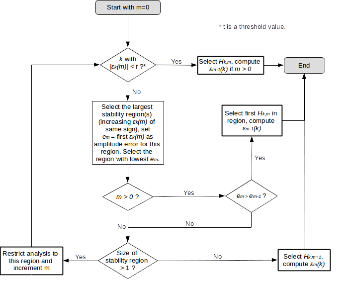
Flowchart to select the “best” value in a Romberg triangle, adapted from the text in M. de Wergifosse et al. Int. J. Quant. Chem. 114, 900 (2014).
Note that the original paper does not give advices on what the threshold value should be, but it clearly depends on the order of magnitude of \(A_d(h)\) and the available (and/or required) precision.
Note
In the case where \(A_d(\mathbf{h}=a^k\mathbf{h}_0)\) is a tensor (because the corresponding function is multivariate), a Romberg triangle must be carried out for each component of this tensor. But since the vector is symmetric, it can reduce the number of components to carry out.
Implementation
The RombergTriangle class implement the Romberg’s triangle algorithm. The constructors expect the value corresponding to increasing k values to be passed as argument.
The \(H_{k,m}\) are available as RombergTriangle.romberg_triangle[k, m]. Note that the values for which \(k \geqslant k_{max} - m\) are set to zero.
The find_best_value() implement the flowchart showed above. To help the (eventual) debugging and understanding, a verbose option is available.
For example, for an univariate function \(F(x)\), compute \(\frac{dF(x)}{dx}\):
a = 2.0
# Forward first order derivative:
c = numerical_differentiation.Coefficients(1, 1, ratio=a, method='F')
derivative_values = []

# compute dF(x) / dx
for k in range(5):
    derivative_values.append(numerical_differentiation.compute_derivative_of_function(
        [(c, 0)],  # derivative with respect to the first (and only) variable
        univariate_function,  # assume defined
        k,
        0.001,  # f0
        1  # R → R
    ))

t = numerical_differentiation.RombergTriangle(derivative_values, ratio=a)
position, value, iteration_error = t.find_best_value(threshold=1e-5, verbose=True)
For a bivariate function \(F(x, y)\), compute \(\frac{\partial^3 F(x, y)}{\partial x \partial y^2}\):
a = 2.0
# centered first and second order derivative:
c1 = numerical_differentiation.Coefficients(1, 2, ratio=a, method='C')
c2 = numerical_differentiation.Coefficients(2, 2, ratio=a, method='C')
derivative_values = []

# compute d³F(x,y) / dxdy²
for k in range(5):
    derivative_values.append(numerical_differentiation.compute_derivative_of_function(
        [(c1, 0), (c2, 1)],  # first and second order derivative with respect to the first and second variable
        bivariate_function,  # assume defined
        k,
        0.001,  # f0
        2  # R² → R
    ))

t = numerical_differentiation.RombergTriangle(derivative_values, ratio=a, r=2)  # r=2 because centered
position, value, iteration_error = t.find_best_value()
Sources
D. Eberly, « Derivative Approximation by Finite Difference ». From the Geometric Tools documentation (last consultation: March 4, 2017).
J.N. Lyness et al. Numer. Math. 8, 458 (1966).
L.F. Richardson et al. Philosophical Transactions of the Royal Society of London. Series A, Containing Papers of a Mathematical or Physical Character 226, 299 (1927).
M. de Wergifosse et al. Int. J. Quant. Chem. 114, 900 (2014).
A.A.K. Mohammed et al. J. Comp. Chem. 34, 1497 (2013).
API documentation
- class qcip_tools.numerical_differentiation.Coefficients(d, p, ratio=2.0, method='C')
Class to store the coefficients for the derivative calculation.
- Parameters:
d (int) – derivation order
p (int) – order of error
ratio (float) – ratio (a)
method (str) – derivation method, either forward (F), backward (B) or centered (C)
- static choose_p_for_centered(d, shift=0)
Choose the precision so that \(d+p-1\) is even (for centered derivatives)
- Parameters:
d (int) – order of the derivative
shift (int) – increase the precision
- prefactor(k, h0)
return the \(\frac{d!}{h^d}\) prefactor, with \(h=a^kh_0\).
- Parameters:
h0 (float) – minimal value
k (int) – Minimal amplitude
- Returns:
prefactor
- Return type:
float
- class qcip_tools.numerical_differentiation.RombergTriangle(values, ratio=2.0, r=1, force_choice=None)
Do a Romberg triangle to lower (remove) the influence of higher-order derivatives.
Note: Romberg triangle indices are n, then k (but printing require n to be column, so invert them !)
- Parameters:
vals (list) – list of derivatives, the first one calculated with the lowest k, the last one the larger
ratio (float) – ratio (a)
r (int) – derivatives to remove. r=1 for backward and forward approximation and 2 for centered approximation.
force_choice (tuple) – force the choice in the Romberg triangle, must be a tuple of the form
(k, m)
- amplitude_error(k=0, m=0)
Compute \(\varepsilon_k(m) = H_{k,m} - H_{k-1,m}\)
- Parameters:
k (int) – amplitude
m (int) – iteration
- Return type:
float
- find_best_value(threshold=1e-05, verbose=False, out=<_io.TextIOWrapper name='<stdout>' mode='w' encoding='utf-8'>)
Find the “best value” in the Romberg triangle
- Parameters:
threshold (float) – threshold for maximum iteration error
verbose (bool) – get an insight of how the value was chosen
- Returns:
a tuple of 3 information: position (tuple), value (float), iteration error (float)
- Return type:
tuple
- iteration_error(m=0, k=0)
Compute \(\varepsilon_m(k) = H_{k,m} - H_{k,m-1}\)
- Parameters:
k (int) – amplitude
m (int) – iteration
- Return type:
float
- romberg_triangle_repr(with_decoration=False, k_min=0)
Print the Romberg triangle …
- qcip_tools.numerical_differentiation.ak_shifted(ratio, q)
Match the \(k\) and the real \(a^k\) value.
For a given \(q\), returns
\[\begin{split}\left\{ \begin{array}{ll} -a^{|q|-1} & \text{if }q<0\\ 0 & \text{if }k=0\\ a^{q-1}&\text{if }q>0 \end{array}\right.\end{split}\]- Parameters:
q (int) – q
ratio (float) – ratio (a)
- Return type:
float
- qcip_tools.numerical_differentiation.compute_derivative_of_function(c, scalar_function, k, h0, input_space_dimension=1, **kwargs)
Compute the numerical derivative of a scalar, calling the appropriate results through
scalar_function, to which the**kwargsparameter is provided.- Parameters:
c (list) – list of tuple to describe the numerical derivative (Coefficient, coordinate)
scalar_function (callback) – a callback function to access the different quantities
k (int) – minimal amplitude
h0 (float) – minimal value
input_space_dimension (int) – dimension of the input vector space
kwargs (dict) – other arguments, transfered to
scalar_function()
- Returns:
value of the derivative (as a scalar)
- Return type:
float
- qcip_tools.numerical_differentiation.real_fields(fields, min_field, ratio)
Return the “real value” of the field applied
- Parameters:
fields (list) – input field (in term of ak)
min_field (float) – minimal field
ratio (float) – ratio
- Return type:
list